
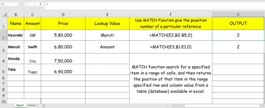
MATCH function is used to find a specified reference value position in a range of cells, and then returns the position of that reference value. Always remember that match function only take a single column or single row as a lookup array(range). Match parameter ( Lookup Value, Lookup array, 0 (For exact match) )
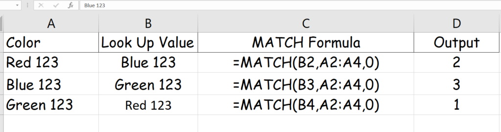
(1) FOR COLUMN DATA Example given below in image.
FORMULA COLUMN: =MATCH(B2,A2:A4,0)
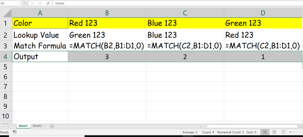
(2) FOR ROW DATA Example given below in image.
FORMULA ROW: =MATCH(B2,B1:D1,0)
Excellent solution.I was looking this from last 3 days but finally I found the solution here. Thank you
Thank you for your valuable comment. Please explore the site for more formula and function for excel.