Please follow the step shown below with images.
This can be used when you want to check or analyze the data with different criteria and luckily excel has two great function to make this possible VLOOKUP 2. SUBTOTAL. Let’s begin.

We have Stock details of LCD, Keyboard, Mouse, Printer etc. From which we need certain types of information separately. Which we will get using VLOOKUP with SUBTOTAL. Follow the steps below.
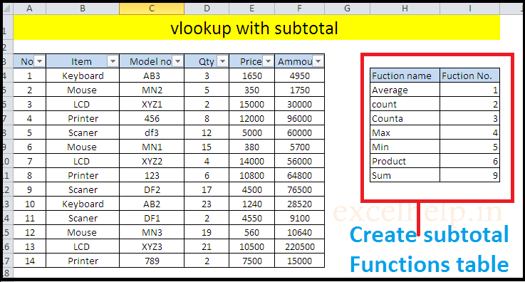
- Create a subtotal Functions table in your worksheet.
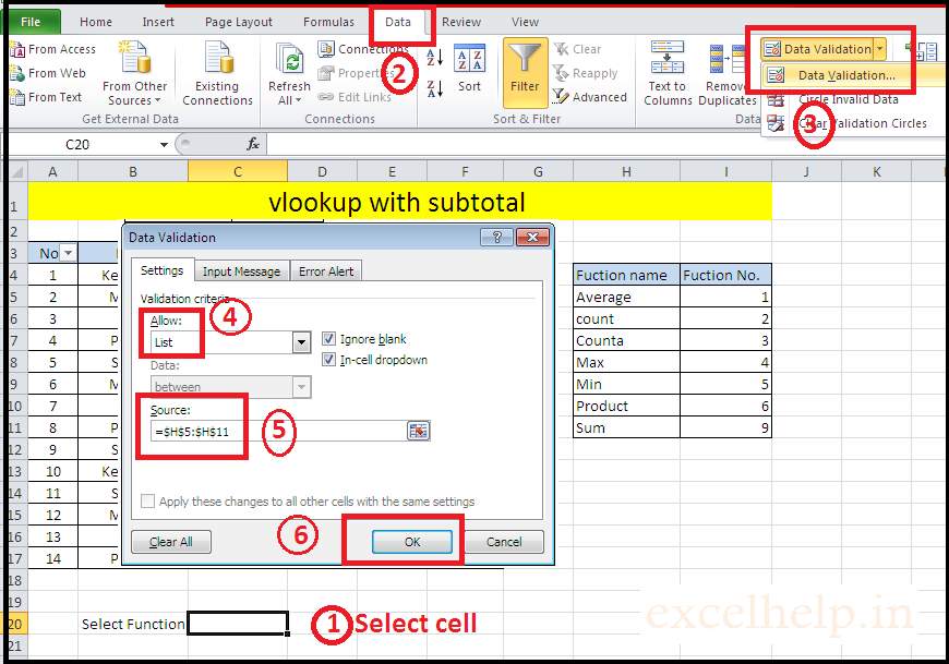
- To create a list of subtotal functions, select cell C20 or according to your choice and adjustment you can change cell until it reference correctly. Then Go to DATA tab >> Data Validation.
- Select list in the dialog box that opens. Select H5:H11 in the source. Click ok.
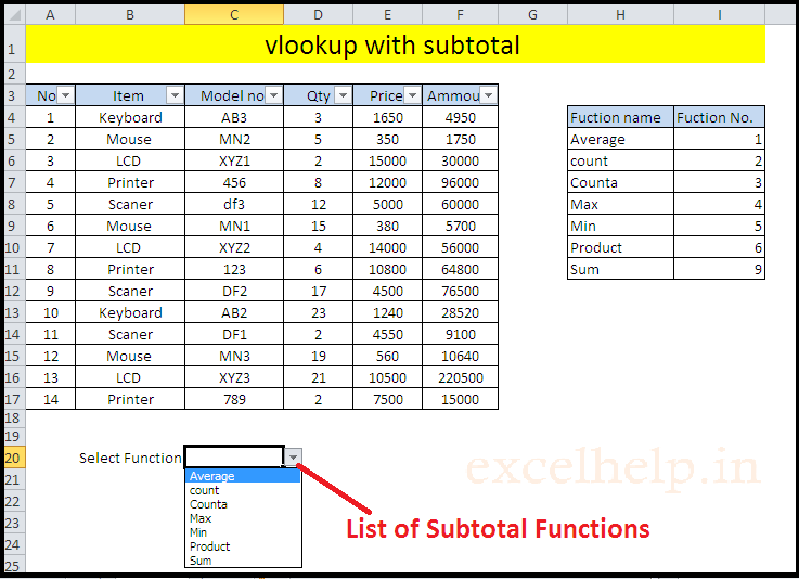
4. The list of various functions of subtotal can be seen in C20.
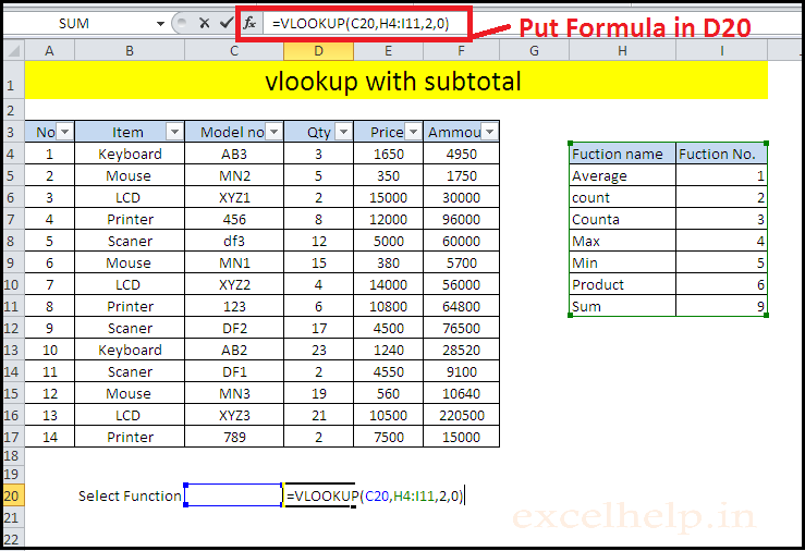
5. Put the formula of VLOOKUP in Cell D20:- =VLOOKUP(C20,H4:I11,2,0)
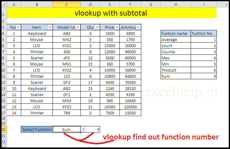
6. So by selecting the function name in the list, VLOOKUP will find the function number in Cell D20.
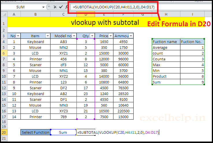
7. Now we will add the subtotal formula into the VLOOKUP formula in Cell D20:- =SUBTOTAL(VLOOKUP(C20,H4:I11,2,0),D4:D17)
8. Now we want to check the stock(Qty) of LCD, Select the LCD using the filter.
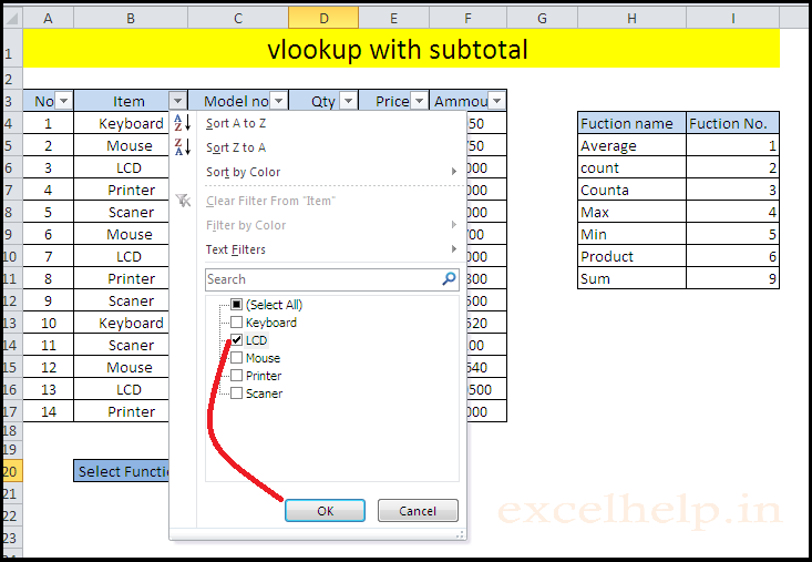
Now Select Sum from the function list. So, you will get the result In Cell D20.
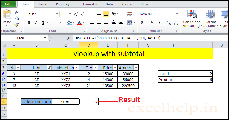
In this example we will try for another subtotal formula..
- Select Count formula from the list
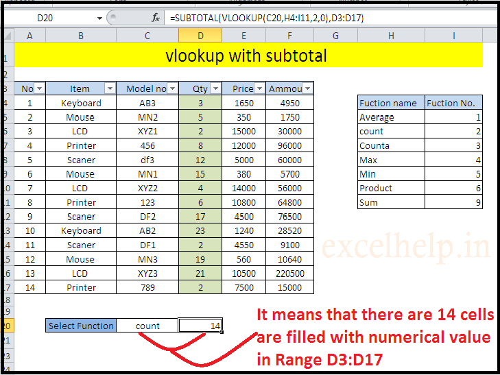
- excel find out howmany cells are filled with numerical value in range D3:D17
