DEPENDENT Drop Down List In Excel

TO create a dependent drop down list please follow the step shown below and example provided with image and video under it.

1. First Select The Reference Cell Where you Want To Have Drop Down List.
2. Then GO To Data Tab.
3. Then Go To Data Validation.
4. One Dialog Box Will Pop-Up.
5. Under That Select The List From Drop Down List.
6. Then Under That In Source Tab Just Provide The Reference Range And Click Ok.
7. Once Your Drop Down List Created Move To Next Column Cell.
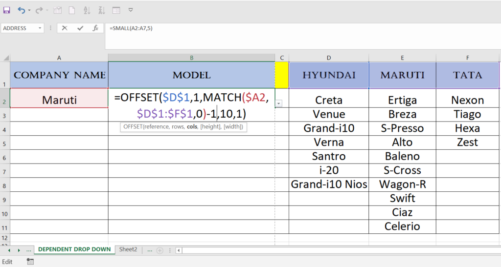
8. Then Again Go To Data Validation And Paste This Formula =OFFSET($D$1,1,MATCH($A2,$D$1:$F$1,0)-1,10,1) And Click Ok.
9. OFFSET FUNCTION:- Offset Function Return A Reference To A Range For The Given Number Of Rows And Columns For The Given Reference.
10. MATCH FUNCTION:- Match Function heck The Position Of A Particular Reference In A Given Array.
11. NOTE:- If You Have A Different Range Please Edit The Formula And Apply The Range According To It.
12. That’s It 🙂

---