NESTED SUMIF With Drop Down List

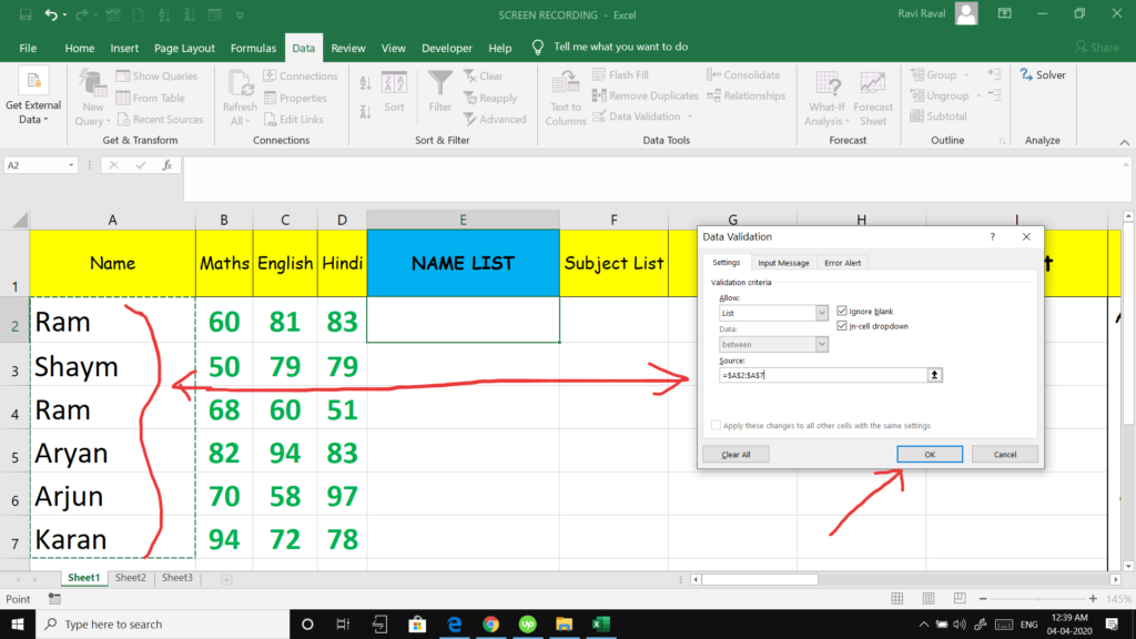
Create a Drop Down List and then apply SUMIF formula in next cell. Just follow the below step to create drop down menu and then apply the Sumif formula

1. First we need to create a drop down list.
2. Select a cell where you want to have your drop down list.
3. Go to Data Tab
4. Go to Data Validation and click on it and one dialog box will pop up.
5. Select List from that dialog box and go down one step into source row in that dialog box.
6. Now select the range for the data you want to create a drop down list. For Ex:- A2:A10
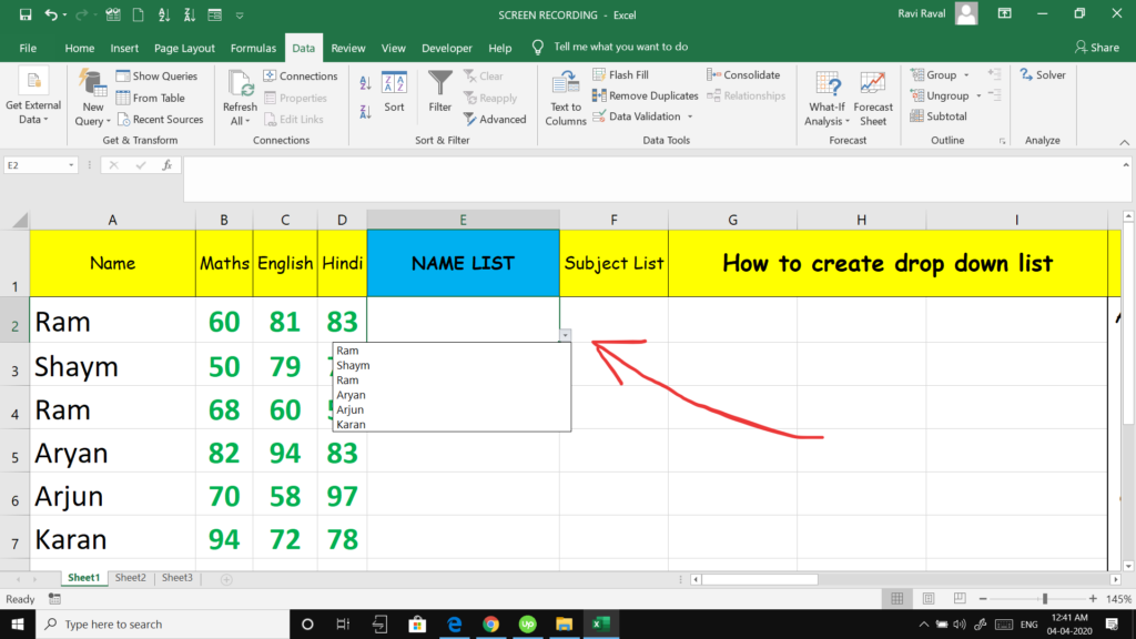
7. Once Selected just hit ok button in the dialog box and your drop down list is prepared.
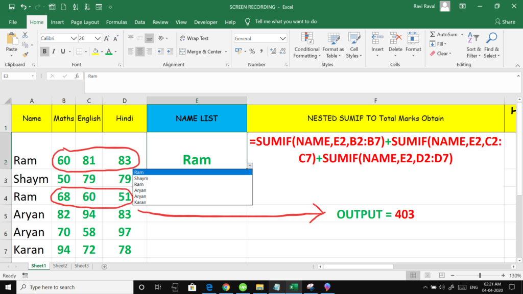
8. Then in the next cell apply the NESTED SUMIF formula.
9. For Example see the step shown in the image and a video provided below.

---