Lookup & Reference Archives - Page 2 of 3

Dec162020 by excelhelp13No Comments

Filter In Excel

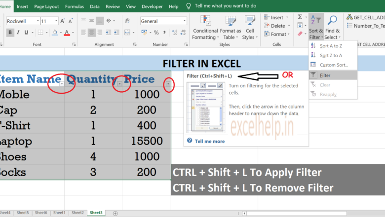
DEFINITION:- Filter is a great way to select the data of your choice by applying to a particular database. Filter has many option available for a different criteria and with the help of those option we can extract the data according to our choice. Filter can be applicable on more then one columns. For more details please follow the step below. Open Excel File.First Select The Database To Apply The Filer.Go To Home Tab.Click On Sort & Filet On The Right Side Under Editing Command Tab.Once Clicked You Will See Drop Down List.Click On Filter Option.Once Clicked The Filer Will Get Applied On Database.Go To The Particular Column For Which You Want The Filter To Look in.Select The Criteria And Apply The Filter.Once Applied Only The Selected Criteria Item Will Be Displayed.For More Deta...

Apr132020 by excelhelp13No Comments

DEPENDENT Drop Down List In Excel

Lookup & Reference

TO create a dependent drop down list please follow the step shown below and example provided with image and video under it. First Select The Reference Cell Where you Want To Have Drop Down List.Then GO To Data Tab.Then Go To Data Validation.One Dialog Box Will Pop-Up.Under That Select The List From Drop Down List.Then Under That In Source Tab Just Provide The Reference Range And Click Ok.Once Your Drop Down List Created Move To Next Column Cell.Then Again Go To Data Validation And Paste This Formula =OFFSET($D$1,1,MATCH($A2,$D$1:$F$1,0)-1,10,1) And Click Ok.OFFSET FUNCTION:- Offset Function Return A Reference To A Range For The Given Number Of Rows And Columns For The Given Reference.MATCH FUNCTION:- Match Function heck The Position Of A Particular Reference In A Given Array.NOTE:- If ...

Apr52020 by excelhelp13No Comments

VLOOKUP In Excel using Different Sheet

FORMULAS, Lookup & Reference

TO use V-lookup on different sheet and extract the data from different sheet please follow the mentioned step below. V-LOOKUP is a vertical lookup formula in excel. V-LOOKUP only looks from left to right. It always take a lookup reference from first column and give result from the column index selected. Let's understand with the example. In this example we need to extract the EMAIL ID From sheet 2 with the help of V-lookup. STEP-1 Select THE CELL STEP-2 =Vlookup( Lookup value , go to sheet 2 and select the table, provide the column index number where Email exist, 0 ( For exact match) HIT ENTER.

Apr32020 by excelhelp13No Comments

SUM Function With OFFSET Function In Excel

FORMULAS, Lookup & Reference, Maths

OFFSET Function is used to move or skip either row or column. Suppose you want to know what data available after every 2 rows or column the offset function is the best choice to get perfect result. It also used with other fucntion available in excel to make it more powerful. For example =SUM(OFFSET(A1,2,2,2,2))

Apr32020 by excelhelp13No Comments

OFFSET Funtion In Excel

FORMULAS, Lookup & Reference

OFFSET Function is used to move or skip either row or column or both. Suppose you want to know what data available after every 2 rows or column the offset function is the best choice to get perfect result. It also used with other available in excel to make it more powerful. For example =Sum(offset(A2,2,3,1,2)

Apr32020 by excelhelp13No Comments

Vlookup with IF Condition

FORMULAS, Logical, Lookup & Reference

When using V-lookup with If logical condition it will determine that when a v-lookup should process and display a result. For Ex: with the help of If condition a user can decide that if a certain value exist then only apply a V-lookup else display a custom message or error. So its very much benefit to use both the function together.

Apr22020 by excelhelp13No Comments

INDIRECT Function In Excel

FORMULAS, Lookup & Reference

INDIRECT function is used in Excel to change over a content string into a legitimate range reference. For example: if you want to find the value of cell A2 then simply use =INDIRECT("a2") or if you have a reference in any cell as we have here in F column simply select that and it will give you the value available in that reference. Clarification: the equation above lessens to =SUM(INDIRECT("a2:c2")). The INDIRECT function add the value of both cells and the content string "a2:c2" converts to a legitimate range reference

Mar312020 by excelhelp13No Comments

INDEX And MATCH Function

FORMULAS, Lookup & Reference

The INDEX MATCH is the combination of two functions in Excel. It looks both the side right and left while Vlookup only lookup in right direction. So its very useful for dynamic lookup reference for the large database. =INDEX() returns the value of a cell in a table based on the column and row number and =MATCH() returns the position of a cell in a row or column.' You can also create a drop down for Product Sku and Model Name / Price

Mar262020 by excelhelp13No Comments

Vlookup And Countif In Excel

FORMULAS, Lookup & Reference

VLOOKUP & COUNTIF -plays a vital role when they both are applied together. Vlookup has limited power. Suppose the lookup value is available more then one time in the specific table or a range then vlookup will pick the the first matching value it found and so as a result you won't get the exact match in some cases or you might be unaware of duplicate value available in a database. Here Countif plays a vital role Countif function check the lookup value in the database and as result it shows how many times that value occurs in a particular database or for a given range. NOTE: The lookup value must be the exact text or numeric number. PARAMETER VLOOKUP: - (Lookup Value, Table Reference, Column Index, 0) 0 - For Exact Match) PARAMETER COUNTIF: - (Range , Criteria) FOR...

Mar172020 by excelhelp132 Comments

MATCH Function In Excel

FORMULAS, Lookup & Reference

MATCH function is used to find a specified reference value position in a range of cells, and then returns the position of that reference value. Always remember that match function only take a single column or single row as a lookup array(range). Match parameter ( Lookup Value, Lookup array, 0 (For exact match) ) (1) FOR COLUMN DATA Example given below in image. FORMULA COLUMN: =MATCH(B2,A2:A4,0) (2) FOR ROW DATA Example given below in image. FORMULA ROW: =MATCH(B2,B1:D1,0)