Home Menu

Mar42023 by excelhelp13No Comments

Number Formats In Excel

Definition:- The Number Format Is A Special Code To Control How Values Are Displayed In Excel. Number Formats Change The Way Numeric Values Are Displayed. But They Do Not Change Actual Values. General - General Option Is The Default Option Applied By Excel For Any Value Number Or Text Format 1. Number:- Number Option Is Used For General Display Of Numbers. The Decimal Number Decimal Can Be Specified. if Want To Display Negative Numbers In Different Formats. 2. Currency:- The Currency Option Can Be Used To Specify Any International Currency Symbol With Numbers. And Also To Specify The Decimal Number. 3. Accounting:- Accounting Option Similar To Currency Option. The Accounting Option Can Set The Currency Symbols And Decimals Together. 4. Date:- With D...

Mar42023 by excelhelp13No Comments

Dynamic Borders in Excel.

Home Menu, tips & Tricks

Excel has an inbuilt Feature to add borders automatically on your worksheet while you are entering value/data in a worksheet. Steps - 1. Select range or entire columns or entire rows or entire sheet. 2. Go to Home tab. 3. Click on Conditional Formatting. 4. Choose New Rule. 5. In the New Formatting Dialogue box, Click on “use a formula to determine Which cells to format” 6. Enter formula in the box- =A1<> “” Note - A1 is a first cell of selection 7. Click on Format 8. Go to Border tab. 9. Click on “outline” 10. Click OK 11. In the New Formatting Dialogue box, Click OK 12. See the Result in below Image. Entering the data automatically adds a border to that cell.

Jun122022 by excelhelp13No Comments

Create diagonal line in cell

Home Menu, tips & Tricks

When you want to show to separate headings within a same cell (one for the row and one for the column), in that case you need to split a cell diagonally. Always remember that cell is a combination of row and column. For Example : Suppose you have data as per image shown below. Now suppose want to insert headings for both column and row in cell A3 for list of name and list of month. STEPS : Select cell A3.Right click on it and Click on format cells...In the format cell dialogue box, go on border tab.Click on diagonal line icon at the bottom right.Click ok. 6. See the result in below image. How to remove diagonal line in excel ? STEPS : Select the cell or cells from which you want to remove the diagonal line.Right click on selection and choose "F...

Jun22022 by excelhelp13No Comments

Move or Copy Sheet in Excel

Home Menu, Menu Bar

When you need to create a new spreadsheet based on an existing one or move a sheet from one excel file to another, you can move or copy a worksheet in the same workbook or another workbook. 1. Move or Copy a worksheet in the same workbook Open the worksheet you want to move or copy.Home > format > move or copy sheet… (you can also open this option using right click on sheet Tab) The Move or Copy dialog box will then open.Choose where you want to place the copy.Click on Create a copy box. (If you don't Click the create a copy box, Excel will only move the sheet.)Click OK. 2. Move or Copy a worksheet to another workbook Open the worksheet you want to move or copy.Home > format > move or copy sheet… (you can also open this opti...

Jun22022 by excelhelp13No Comments

Protect Worksheet in Excel

Home Menu, Menu Bar

When you share an Excel file with other users, you may want to protect a worksheet to help prevent it from being changed. Using this option, you can lock your Excel sheet with a password and you can make only certain parts of the sheet editable and users will not be able to modify data in any other region in the sheet. Preview in new tab How to Protect Sheet in Excel ? Steps:- Right click on sheet tab > Click Protect Sheet. Or Home> Format > Protect Sheet Check on protect worksheet and content of locked cells box.Enter a password.Check the actions you allow the users of your worksheet to perform.Note:- if you don't check any action, users can only view the Excel file.Click OK. Confirm the password and click OK.Your worksheet is protect...

Jun22022 by excelhelp13No Comments

Strikethrough Effect in Excel

Home Menu, Menu Bar

Strikethrough Effect is Useful for drawing a line in the center above the data / text in the cell to mark it as a completed or to display as depricated or non use as per the needs vary. How to Insert Strikethrough Effect in Excel ? For Example:- excelhelp.in Steps:- Select DataClick Home tab > format > Format cell… or right click on any cell > Format cell… The format cell dialog box will open.Click on font tab > font effectCheck on Strikethrough box.Click OK How to Remove Strikethrough Effect in Excel ? Select the data.Click Home tab > format > Format cell… OR right click on any cell > Format cell… The format cell dialog box will open.Click on font tab > font effectUnCheck on Strikethrough box.Click OK

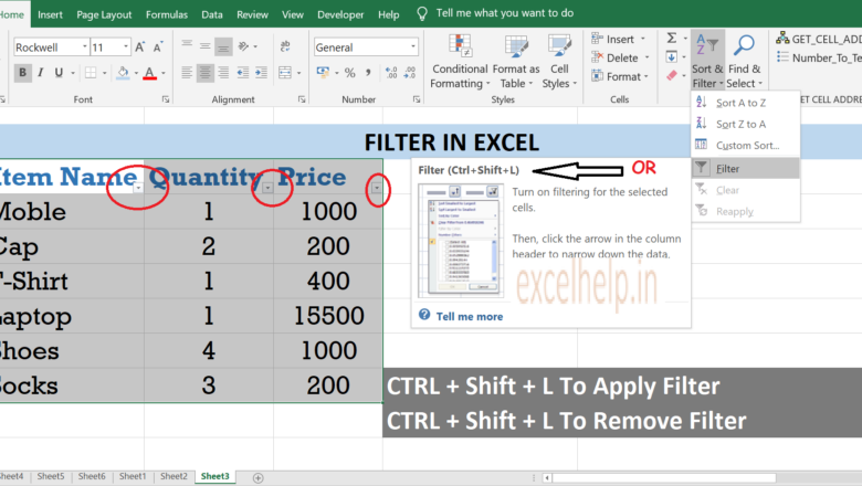
Dec162020 by excelhelp13No Comments

Filter In Excel

Home Menu, Lookup & Reference

DEFINITION:- Filter is a great way to select the data of your choice by applying to a particular database. Filter has many option available for a different criteria and with the help of those option we can extract the data according to our choice. Filter can be applicable on more then one columns. For more details please follow the step below. Open Excel File.First Select The Database To Apply The Filer.Go To Home Tab.Click On Sort & Filet On The Right Side Under Editing Command Tab.Once Clicked You Will See Drop Down List.Click On Filter Option.Once Clicked The Filer Will Get Applied On Database.Go To The Particular Column For Which You Want The Filter To Look in.Select The Criteria And Apply The Filter.Once Applied Only The Selected Criteria Item Will Be Displayed.For More Detai...

Dec112020 by excelhelp13No Comments

Goto Special In Excel

Home Menu, Menu Bar

DEFINITION:- The Go To Special Function In Excel Allows You To Quickly Select All Cells That Meet Certain Criteria, Such As Cells Containing: Comments, Constants, Formulas (Numbers, Text, Logical, Errors), Blank Cells, Objects Etc. Blank Will Select The Blank Cell Only.Current Region Will Select From The Active Cell To Last Row. makes Sure You Don't Have A Blank Cell Otherwise It Will Consider Above The Blank Row As Last Row.Current Array Will Select The Active Range Belongs To.Object Will Select Any Object Available In A Range. Ex:- ShapesLast Cell Will Select The Last Used Cell In A Worksheet. Even If You Delete The Data From Cell.Visible Cells Will Select Only Visible Cell If Any Filter Is Applied Or Even Any Row Or Columns Are Available.Conditional Formatting Will Select The Format...

Dec112020 by excelhelp13No Comments

Go To Method In Excel

Home Menu, Menu Bar

Definition:- Go To Feature Is Use To Move The Cell Cursor To A New Cell In The Worksheet. You Can Also Use This Feature To Select A Range Of Cells. There Are Three Ways To Access “Go To” Press The F5Press Ctrl+GHome Tab – Find & Select – Choose “Go To…” To Move The Cell Cursor To A Particular Cell, Enter The Cell Address In The “Reference” Text Box And Click Ok. You Can Also Select A Range Of Cells By Taking These Steps: Select The First Cell Of The Range.Type The Cell Address Of The Last Cell In The Range In The “Reference” Text Box.Hold Down The Shift Key As You Click Ok Or Press Enter To Close The Go To Dialog Box.

Dec102020 by excelhelp13No Comments

How To Use Find And Replace In Excel

Home Menu, Menu Bar

FIND : Click CTRL + F One Find And Replace Dialog Box Will PopupSelect Database Or Range Or Directly Type The Text Or Number To Find Out OR Follow The Below Step For Another Method.Click The Home TabGo To The Editing Group Command Tab.Click On Find & Select ButtonA Dropdown Menu Will Appear. Click On Find. Steps :- In The Dialog Box Input The Text Or Number In “Find What” To Find The Data Within The Worksheet Or Database For And Then - Click “Find Next” MULTIPLE SEARCH : If You Want To Find Out How Many Times A Particular Word Or Phrase Has Been Used Or Found In Your Database Or Worksheet , Click “Find All” In The Dialog Box Will Populate The Match Row Where The Query Data Is Available. FIND & REPLACE : Select Database Or RangeClick The Home TabG...