
Pivot Table is used to summarize and organize the data of extensive table. This includes sums, count, average or any other data statistics. Pivot table groups and organize data in a presentable way. Pivot tables are most used to sort out the data and prepare a summarize report in just few seconds.
To create a pivot table and generate a summarize report please follow the step mentioned below.
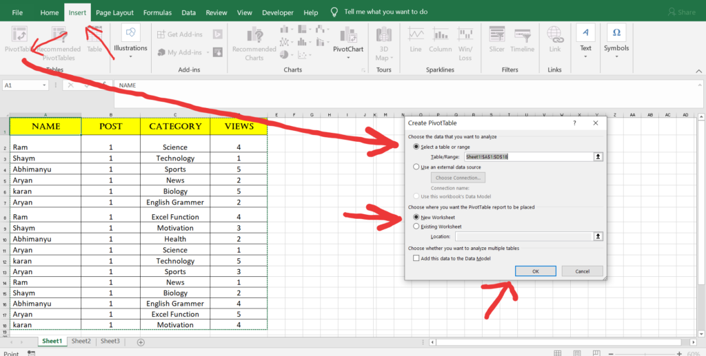
- First Go To Insert Tab available on top ribbon of excel sheet.
- Then click on Pivot Table
- Once clicked a Dialog Box will pop-up.
- In the select range source bar it will automatic select the source table. But if you want to select the different range you can select it.
- Then little down in that dialog box you will find 2 option to select the sheet (1) New Sheet (2) Existing Sheet.
- If you select New Sheet and click ok button it will automatically create a table on a New Sheet.
- If you choose Existing Sheet you will need to give the location below it. Select any single cell and click ok button.
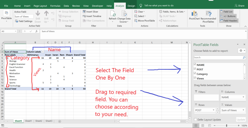
- Then you will find a Pivot Table fields on the right side of the sheet and under it you will find Filter – Column – Rows – Values.
- Filter is used to filter the data.
- Column is used to display the data Column wise
- Row is use to display the data Row wise
- Value is use to count – sum – or other operation.
- Last step – Select the Pivot Fields and drag to the relative areas.
- For more details see the example provided below in image and video.