
How to use and apply the Top / Bottom rules in conditional formatting please follow the step shown below and example in image and video.
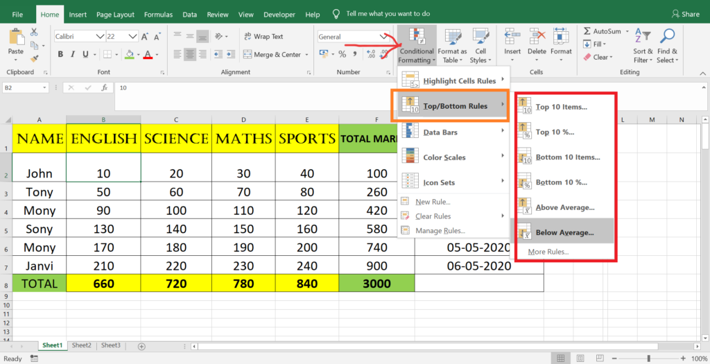
TOP 10 ITEMS:- When you apply this highlighting rule it will highlight the top 10 highest number from the table range.
TOP 10%:- When you apply this highlighting rule it will highlight the top 10% of the table count cell. Suppose there are 24 cell are there in a selected table and 10% of 24 is 2.4% then it will highlight 2 top value of the entire table range.
BOTTOM 10 ITEMS:- When you apply this highlighting rule it will highlight the bottom 10 lowest number from the table range.
BOTTOM 10%:- When you apply this highlighting rule it will highlight the bottom 10% of the table count cell. Suppose there are 24 cell range selected and 10% of 24 is 2.4% then it will highlight 2 bottom value of the entire table range.
ABOVE AVERAGE:- When you apply this highlighting rule it will highlight the number which are above the average of entire table range.
BELOW AVERAGE:- When you apply this highlighting rule it will highlight the number which are below the average of entire table range.
NOTE:- You can apply this all formatting to analyze the top 10 days sales, top 10 students or sales person or anything.