CONDITIONAL FORMATING In Excel

To Use And Apply The Conditional Formatting Please Follow The Step Shown Below And Example In Image And Video.

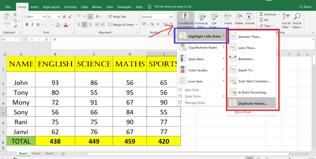
1. HIGHLIGHT GREATER THAN:- When you apply this greater than highlighting rule it will highlight the number which is greater than the reference number.
2. LESS THAN:- When you apply this less than highlighting rule it will highlight the number which is less than the reference number.
3. BETWEEN:- When you apply this between highlighting rule it will highlight the number which is are between the given two reference number.
4. EQUAL TO:- When you apply this equal to highlighting rule it will highlight the number which is equal to or same to reference number.
5. TEXT THAT CONTAINS:- When you apply this text to contains highlighting rule it will highlight the text from the selection which contain exact text as reference text.
6. A DATE OCCURING:- When you apply this date occuring highlighting rule it will highlight the the date according to the given reference date or a specific period.
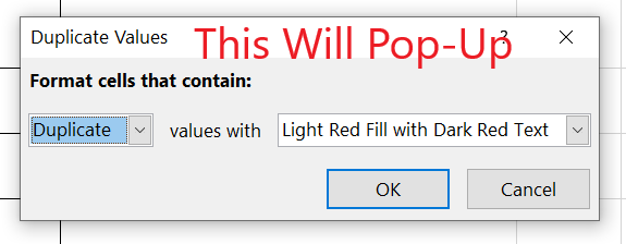
7. DUPLICATE VALUE:- When you apply this duplicate highlighting rule it will highlight the the value which are found duplicate exactly as given reference text or a value for the selected range.