
To Highlight The Negative And Positive Number Automatically In Excel Please Follow The Step & Images Shown Below.
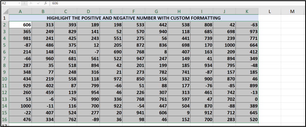
- SELECT THE RANGE
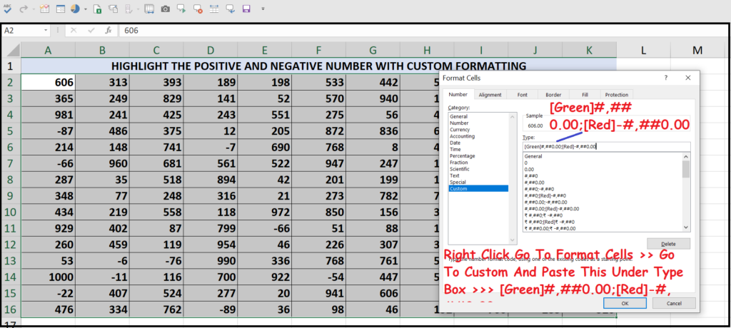
- RIGHT CLICK >> GO TO FORMAT CELLS >> THEN GO TO CUSTOM FORMAT & PASTE THIS UNDER TYPE BOX :- [Green]#,##0.00;[Red]-#,##0.00
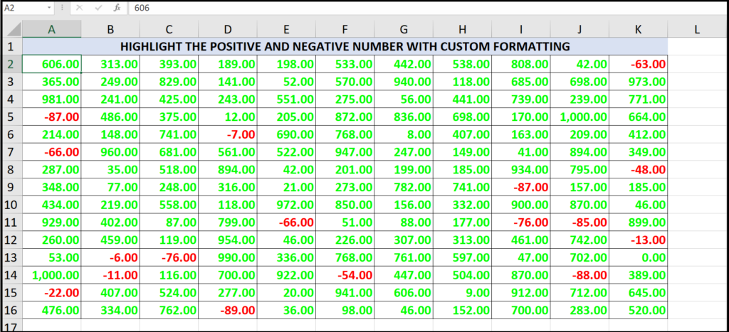
- NOW YOU WILL SEE THE GREEN FONT FOR POSITIVE NUMBER & RED FONT FOR NEGATIVE NUMBER.
- IF NOW YOU CHANGE ANY NUMBER AND IF IT IS NEGATIVE IT WILL CHANGE TO RED AND IF IT IS POSITIVE IT WILL CHANGE TO GREEN.
- NOTE: THIS ONLY WORK FOR THE SELECTION RANGE. SO PLEASE MAKE SURE TO SELECT THE RANGE PROPERLY OR SELECT THE WHOLE SHEET CELLS BEFORE APPLYING THE CUSTOM FORMAT.