Conditional Highlight Negative And Positive Cell In Excel

To Highlight Positive Or Negative Number We Can Use Conditional Formatting. Please Follow The Step Shown Below.

1. First Select The Range Were You Want To Apply The Conditional Formatting. Example : A2:F10
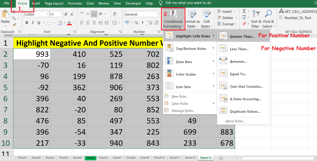
2. Then Go To Home Tab.
3. Click On Conditional Formatting.
4. Select Highlight Cell Rules.
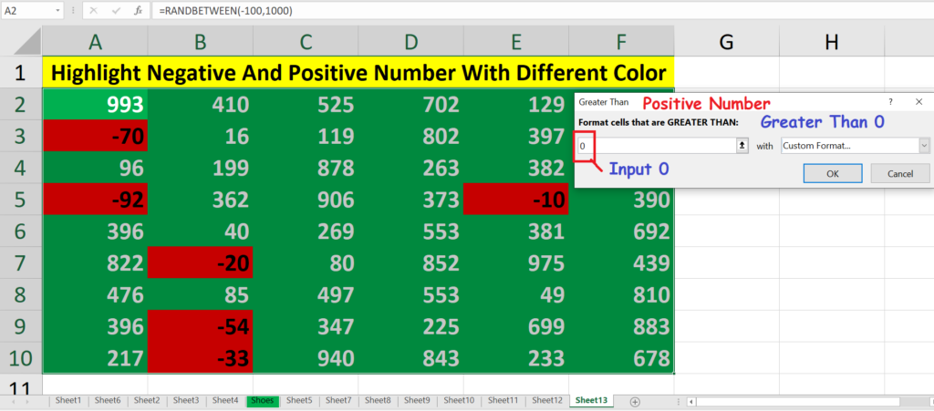
5. To Highlight The Positive Number Click On Greater Than.
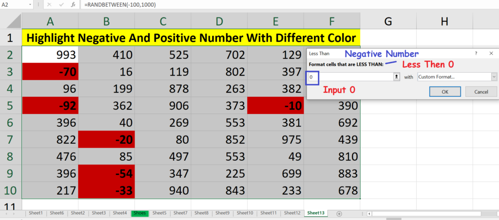
6. To Highlight The Negative Number Click On Less Than.
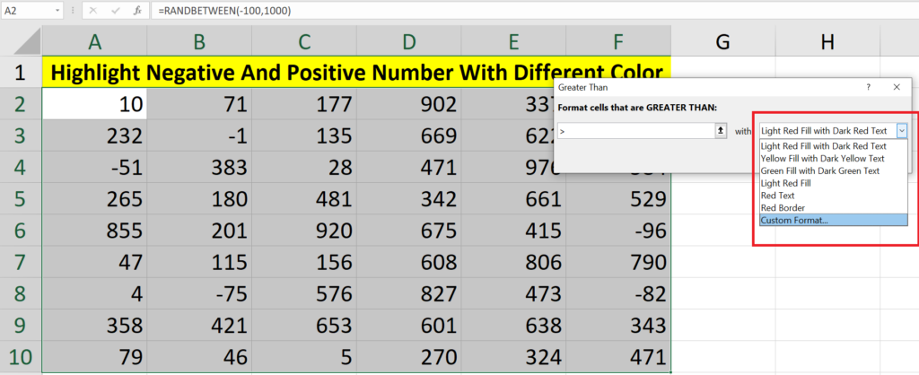
7. One Dialog Box Will Pop-Up To Enter The Value As Per Need,
8. For Positive Number Add 0. ( In Greater Than. )
9. For Negative Number Add 0 ( In Less Than. )
10. For Custom Format Select Custom From Drop Down List On Right Hand Side.
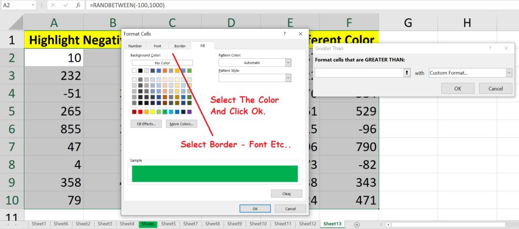
11. You Can Apply Many Formatting Like Font Color – Border – Cell Color Etc..
12. Once Done Click Ok.
13. Now you Must See the Applied formatting On A The Cells.
14. Now If you Change The Number The Formatting Will Also Get Change According To The Applied Rule And Conditions.
15. NOTE: You Can Apply As Many Condition As you Want.
16. For In Detail Please Check This Post. CONDITIONAL FORMATTING.
17. That’s It 🙂
18. Please Check The Image Below.