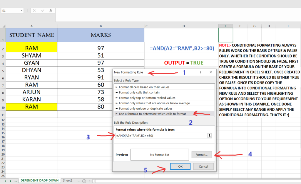
How to use and apply the Conditional Formatting rules by using custom formulas please follow the step shown below and example in image and video.
- NOTE:- Conditional Formatting Rules Always Work On The Basis Of True & False Only.
- Whether The Condition Should Be True Or Condition Should Be False.
- First Create A Formula On The Base Of Your Requirement In Excel Sheet.
- Once Created Check The Result It Should Be Either True Or False.
- Now Select The Range Of Your Data.
- GO To Home Tab
- Then Go To Conditional Formatting.
- Then Click & Select New Rule.
- One Dialog Box Will Pop-Up
- Then Select Use A Formula – Last In Option List.
- Type The Formula In Rule Description Or Paste The Formula You Already Created In Excel Sheet.
- Once Its Done Select The Formatting Option According To Your Requirement As Shown In This Example.
- Once It’s Done lick Ok.
- That’s It 🙂

